本文参考华泰证券《华泰风险收益一致性择时模型》,采用研报内的方法对风险收益一致性进行研究。根据研报分析,当行业的收益率与其贝塔呈现较好的正相关时,可以认为市场收益率为正,市场处于上涨状态;当行业的收益率与其贝塔呈现负相关时,可以认为市场收益率为负,市场处于下跌状态,利用这种关系即可构造择时模型。这是华泰风险收益一致性择时的基本思想。
根据此结论,本文试图对研报里面的结果进行了复现并分析,并对风险收益一致性进行了研究,从而其构建择时信号。另外,本文还试图将风险收益一致性信号与均线信号相结合,探究均线策略能否进一步改善风险收益一致性策略。
自从20世纪50年代资本资产定价模型提出之后,人们习惯使用贝塔来代表资产与市场组合之间的关系。根据资本资产定价模型,假设资产的贝塔值是稳定的,那么在市场上涨的时候,贝塔高的资产应该收获更高的收益,但是市场下跌的时候也会承担更多的损失,所以贝塔值代表了资产承担市场风险的大小。通过资本资产定价模型我们找到了市场中存在的一种结构,不同资产的涨跌幅与市场组合的涨跌幅会存在相对固定的对应关系。如果反 过来使用这种对应关系,就得到了一种观察市场的方法,比如当发现高贝塔的资产收益较高,低贝塔的资产收益较低时,那市场大概率处于一种上升状态,当发现高贝塔的资产收益较低,低贝塔的资产收益较高时,市场可能处于一种下跌状态,如此我们可以构造一个择时模型。
贝塔是一项资产或投资组合对市场投资组合方差 的贡献程度,也即该资产或组合相对于市场波动性的敏感程度。贝塔越高,表明该资产或 组合受市场波动的影响越大,从而带来更大的风险溢价(即$β_p(R_m-R_f)$,括号内的部分为市场风险溢价)。在市场上涨(或下跌)时,高贝塔的资产由于承担了更多的市场风险, 其收益的变动会比低贝塔的资产更为剧烈。
在资本资产定价模型的收益率公式中,如果贝塔是固定的,那资本的收益率主要取决于市场的收益率,所以市场上涨高贝塔行业涨幅更大,市场下跌同样高贝塔行业会下跌更多。借助于这一点,可以尝试逆向推断市场的涨跌,当行业涨幅与其贝塔状态基本一致的时候说明市场是上涨的,相反的时候说明市场是下跌的。
研报中市场指数选用万得全A指数,行业指数选用中信一级行业指数。由于数据来源限制,此处行业指数我们选择申万一级行业指数,而市场指数选取国证全A指数。数据时间段为2005年2月3日至今,频率为周度。我们需要用指数的周收益率来计算beta。
#数据获取
from jqdata import *
import time,datetime
import numpy as np
import pandas as pd
from jqdata import finance

# #获取每周最后一个交易日的申万一级行业指数收盘价
industries_df = get_industries("sw_l1")
deprecated_industries = ['801060','801070','801090','801100','801190','801220']
industries = list(industries_df.index)
start_dates = list(industries_df['start_date'])
trade_days = get_trade_days(start_date='2005-02-03')
ret_dict={}
for code,start_date in zip(industries,start_dates):
    if code in deprecated_industries:
        continue
    #国证A指在2005年2月3日后才有数据
    start_date = trade_days[0]
    q=query(finance.SW1_DAILY_PRICE).filter(finance.SW1_DAILY_PRICE.date>=start_date,finance.SW1_DAILY_PRICE.code==code)
    df=finance.run_query(q)
    if len(df)!=len(trade_days):
        trade_days=trade_days[0:-1]
    df_date=list(df['date'])
    df_date_weekday =np.array([i.weekday() for i in df_date])
    b=df_date_weekday[0:-1]-df_date_weekday[1:]
    c=df['date']
    close=np.array(df[0:-1][b!=-1]['close'])
    ret = close[1:]/close[:-1]-1
    ret_dict[code]=ret

ret_dict['date'] = df[0:-1][b!=-1]['date'][1:]

#获取每周最后一个交易日的国证A指
mkt_index = get_price('399317.XSHE',start_date='2005-02-03',end_date=trade_days[-1],fields=['close'])
mkt_close = np.array(mkt_index[0:-1][b!=-1]['close'])
mkt_ret =mkt_close[1:]/mkt_close[0:-1]-1
ret_dict['mkt'] = mkt_ret
ret_df = pd.DataFrame(ret_dict)

ret_df.head(10)
| 801010 | 801020 | 801030 | 801040 | 801050 | 801080 | 801110 | 801120 | 801130 | 801140 | 801150 | 801160 | 801170 | 801180 | 801200 | 801210 | 801230 | 801710 | 801720 | 801730 | 801740 | 801750 | 801760 | 801770 | 801780 | 801790 | 801880 | 801890 | date | mkt | |
|---|---|---|---|---|---|---|---|---|---|---|---|---|---|---|---|---|---|---|---|---|---|---|---|---|---|---|---|---|---|---|
| 4 | 0.016752 | -0.000055 | -0.002821 | -0.019222 | 0.004743 | 0.003767 | -0.001150 | -0.008497 | 0.008307 | -0.003766 | 0.000467 | -0.005438 | -0.014379 | -0.011145 | 0.003902 | -0.004498 | 0.003895 | -0.000345 | 0.013141 | 0.005468 | 0.010417 | -0.005446 | -0.003698 | -0.004274 | -0.024481 | -0.003074 | -0.008177 | 0.002992 | 2005-02-18 | -0.004816 |
| 9 | 0.063175 | 0.053068 | 0.059062 | 0.035376 | 0.074910 | 0.049745 | 0.056839 | 0.049664 | 0.053907 | 0.047423 | 0.048626 | 0.038252 | 0.034873 | 0.034023 | 0.058412 | 0.070708 | 0.063751 | 0.058779 | 0.058697 | 0.079068 | 0.067695 | 0.077919 | 0.070035 | 0.030865 | 0.024434 | 0.037494 | 0.040080 | 0.056129 | 2005-02-25 | 0.048701 |
| 14 | -0.002303 | -0.029427 | -0.014190 | -0.032868 | -0.016789 | -0.024223 | -0.034625 | -0.015581 | -0.017670 | -0.025470 | -0.017187 | 0.000461 | -0.014089 | -0.024456 | -0.023079 | 0.001736 | -0.022184 | -0.029780 | -0.011949 | -0.027190 | -0.027025 | -0.023410 | -0.013838 | -0.009385 | -0.037843 | -0.025196 | -0.040671 | -0.022206 | 2005-03-04 | -0.020454 |
| 19 | -0.011705 | -0.018241 | 0.015400 | 0.005215 | 0.019510 | 0.011692 | 0.018466 | 0.010708 | -0.000124 | -0.006557 | 0.018899 | -0.003516 | 0.026794 | -0.011475 | 0.019286 | 0.024578 | -0.007614 | 0.008692 | 0.008764 | -0.003585 | 0.001311 | 0.014821 | -0.004886 | -0.012585 | -0.030693 | -0.035479 | -0.009785 | 0.012533 | 2005-03-11 | 0.005118 |
| 24 | -0.057641 | -0.048873 | -0.052910 | -0.032943 | -0.060030 | -0.083581 | -0.073817 | -0.013138 | -0.056484 | -0.051227 | -0.052252 | -0.058472 | -0.033417 | -0.076386 | -0.045483 | -0.046424 | -0.063510 | -0.057643 | -0.041514 | -0.063254 | -0.032789 | -0.073470 | -0.072627 | -0.046506 | -0.014085 | -0.073533 | -0.077500 | -0.056094 | 2005-03-18 | -0.052057 |
| 29 | -0.001022 | -0.004992 | -0.013292 | -0.018703 | -0.010654 | -0.046608 | -0.035764 | -0.005726 | -0.020882 | -0.031384 | -0.012118 | -0.024944 | 0.007835 | -0.017959 | -0.020444 | -0.016896 | -0.027020 | -0.017283 | -0.018855 | -0.007214 | -0.014308 | -0.046290 | -0.037950 | -0.042745 | -0.022360 | -0.051607 | -0.029573 | -0.014648 | 2005-03-25 | -0.018570 |
| 34 | -0.010949 | 0.043812 | 0.014796 | 0.027020 | -0.010944 | 0.009051 | 0.009485 | 0.016377 | -0.021537 | 0.012236 | 0.000475 | 0.014555 | 0.010731 | -0.000426 | 0.002580 | -0.009217 | -0.012868 | -0.000944 | -0.005312 | -0.000228 | -0.009677 | 0.003298 | 0.002245 | 0.003748 | 0.030967 | 0.028782 | -0.011591 | -0.005097 | 2005-04-01 | 0.007781 |
| 39 | 0.012764 | 0.043675 | 0.039942 | -0.016439 | 0.043137 | 0.001708 | 0.010010 | 0.026947 | 0.022241 | 0.003975 | 0.028170 | 0.026602 | 0.034663 | 0.023625 | 0.035504 | 0.044257 | 0.040609 | 0.017659 | 0.030992 | 0.006308 | 0.030041 | 0.009610 | -0.003075 | -0.005335 | 0.072019 | 0.053887 | 0.013579 | 0.037236 | 2005-04-08 | 0.024562 |
| 44 | -0.039831 | -0.045880 | -0.026454 | -0.009985 | -0.042549 | -0.042376 | 0.000901 | -0.032222 | -0.035573 | -0.005496 | -0.030181 | -0.031662 | -0.032850 | -0.037683 | -0.036499 | -0.024911 | -0.050571 | -0.044134 | -0.043749 | -0.022515 | -0.032306 | -0.051727 | -0.045429 | -0.050117 | -0.032454 | -0.021380 | -0.025137 | -0.031692 | 2005-04-15 | -0.032726 |
| 49 | -0.077672 | -0.006006 | -0.054275 | -0.031983 | -0.050219 | -0.093586 | -0.044920 | -0.037758 | -0.057848 | -0.061305 | -0.039812 | -0.049278 | 0.000008 | -0.069730 | -0.040218 | -0.069477 | -0.077392 | -0.085568 | -0.047821 | -0.057839 | -0.046698 | -0.078703 | -0.090011 | -0.029196 | -0.018651 | -0.061226 | -0.074159 | -0.067677 | 2005-04-22 | -0.047760 |
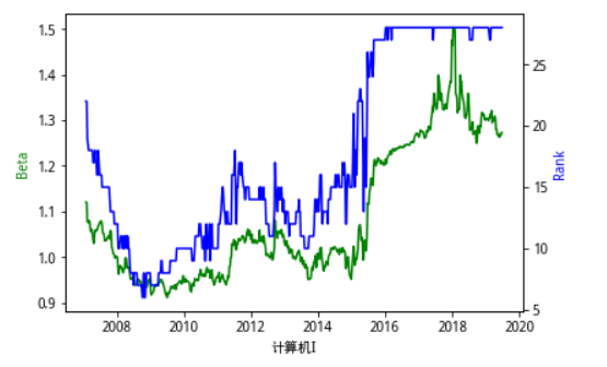
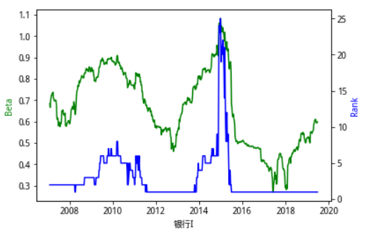
为了直观地感受不同行业Beta值地周期特征,我们将行业贝塔在每一个截面从小到大排序,得到行业贝塔的秩次,用 rank 表示。将行业贝塔rank在同一张图中表示出来,得到下面这一系列的图。总的来看,行业beta值比较稳定,但在某些特殊时刻也存在跃迁 式的变化。例如 15 年中期,急剧的上涨行情使很多行业的贝塔发生了变化,而且这种变化也延续至今。偏向于 TMT类型的行业,计算机、传媒、电子、通信、电力设备等在15年5、6月份贝塔值急剧上升,转变为高贝塔类行业,而银行、非银等行业贝塔值快速下降,行业特性向低贝塔靠近,在此之后,行业的贝塔值在16年一直处于比较稳定的状态。
import statsmodels.api as sm
#用N周的数据计算Beta,第N周开始有beta,研报中N为98

#获取行业中文名称
ind_df=get_industries('sw_l1')
ind = ind_df.index
valid_ind = list(set(ind)^set(deprecated_industries))
valid_ind_df = ind_df.loc[valid_ind]
ind_dict = dict(zip(valid_ind_df.index,valid_ind_df['name']))

#计算行业beta
N=98
beta_dict = {}
beta_dict['date'] = ret_dict['date'][N-1:]
for k,ret in ret_dict.items():
    if k!='date'and k!='mkt':
        beta_series = []
        for i in range(len(ret)-N+1):
            x = sm.add_constant(mkt_ret[i:i+N])
            model = sm.OLS(ret[i:i+N],x)
            results = model.fit()
            beta_series.append(results.params[1])
        beta_dict[k] = beta_series

beta_df = pd.DataFrame(beta_dict)
date = beta_df['date']
beta_df_t = beta_df.T
beta_rank=beta_df_t.iloc[1:].rank().T
plt.figure()
for i in range(1,29):
    print(i)
    #plt.subplot(28,1,i)
    plt.figure(figsize=(10,8))
    code = beta_df.columns[i]
    x = beta_dict['date']
    y1 = beta_dict[code]
    y2 = beta_rank[code]
    fig, ax1 = plt.subplots()
    ax2 = ax1.twinx()
    ax1.plot(x,y1,'g-')
    ax2.plot(x,y2,'b-')
    ax1.set_xlabel(ind_dict[code])
    ax1.set_ylabel("Beta",color='g')

    ax2.set_ylabel("Rank",color='b')

    plt.show()
1
<Figure size 432x288 with 0 Axes>
<Figure size 720x576 with 0 Axes>

2
<Figure size 720x576 with 0 Axes>

3
<Figure size 720x576 with 0 Axes>

4
<Figure size 720x576 with 0 Axes>

5
<Figure size 720x576 with 0 Axes>

6
<Figure size 720x576 with 0 Axes>

7
<Figure size 720x576 with 0 Axes>

8
<Figure size 720x576 with 0 Axes>

9
<Figure size 720x576 with 0 Axes>

10
<Figure size 720x576 with 0 Axes>

11
<Figure size 720x576 with 0 Axes>

12
<Figure size 720x576 with 0 Axes>

13
<Figure size 720x576 with 0 Axes>

14
<Figure size 720x576 with 0 Axes>

15
<Figure size 720x576 with 0 Axes>

16
<Figure size 720x576 with 0 Axes>

17
<Figure size 720x576 with 0 Axes>

18
<Figure size 720x576 with 0 Axes>

19
<Figure size 720x576 with 0 Axes>

20
<Figure size 720x576 with 0 Axes>

21
<Figure size 720x576 with 0 Axes>

22
<Figure size 720x576 with 0 Axes>

23
<Figure size 720x576 with 0 Axes>

24
<Figure size 720x576 with 0 Axes>

25
<Figure size 720x576 with 0 Axes>

26
<Figure size 720x576 with 0 Axes>

27
<Figure size 720x576 with 0 Axes>

28
<Figure size 720x576 with 0 Axes>

接下来我们利用行业的贝塔与其收益率之间的关系构建择时模型,由于贝塔代表行业相比于市场组合的风险承担,本质上也代表行业相对于市场组合的杠杆率,一定程度上度量了风险,所以将择时模型起名为风险收益一致性择时模型。
如前所述,资产的贝塔大小与资产收益变动幅度存在相关性,而各个行业具有特征明显且相对稳定的贝塔。基于这一性质,我们可以对行业的贝塔与收益进行观测,进而对判断市场的运行状况:
1、当贝塔与收益趋于一致,即高贝塔的行业收益更高时,认为市场表现良好,观点看多;
2、当贝塔与收益呈反向关系,即高贝塔的行业收益更低时,认为市场表现不佳,观点看空。这一策略有着清晰的逻辑,并且以行业与市场指数做比较,在长期看较为稳定,适合对市 场进行长期判断。
为了度量行业贝塔与收益的一致性,我们引入Spearman 秩相关系数作为工具。
我们利用Spearman秩相关系数度量行业Beta与收益的一致性。
利用之前两年左右的数据,我们在每周末可以得到28个行业的Beta。得到Beta后,我们计算行业Beta与行业收益率的秩相关系数。在计算时,我们假设行业贝塔在周中保持静态不变,采用29个行业当周的收益率$r_t$与上周的贝塔 $β_{t-1} $进行计算。这样的好处是贝塔中并没有包含本周的收益率信息,两者保持一定意义上的相对独立,防止某个异常值带来的贝塔偏离。
为了过滤相关系数中的噪音,得到更稳定的长周期择时信号,我们对秩相关系数取4周的滑动平均,得到滑动平均序列 𝜌̅𝑠。
根据研报,我们选取98周数据计算β,秩相关系数选取0.128作为阈值。当𝜌̅𝑠>0.128时,发出一次买入信号;当𝜌̅𝑠<-0.128时,发出一次卖出信号。若连续发出两次同向信号,则执行买入/卖出操作。
从信号发出的时间来看,使用不同的行业指数对于信号发出还是有些影响的。总的来说,使用申万行业一级指数和研报中阈值的结果不佳,年化收益过低,不能跑赢国证A指。
from scipy.stats import spearmanr
threshold=0.128

#threshold为阈值,print_order为是否打印买卖指令
def back_test(threshold,print_order=True):
    corr_list =[]
    #第t周收益与t-1周的beta
    for i in range(len(beta_df)-1):
        corr_list.append(spearmanr(beta_df.iloc[i][1:].astype(float),ret_df.iloc[i+N][:-2].astype(float))[0])
    corr_dict={}
    corr_dict['date']=beta_df['date'][1:]
    corr_dict['corr']=corr_list
    corr_df=pd.DataFrame(corr_dict)
    corr_df['ma_4'] = corr_df['corr'].rolling(window=4,min_periods=1).mean()
    corr_df['signal']=0
    corr_df['signal'][corr_df['ma_4']>threshold]=1
    corr_df['signal'][corr_df['ma_4']<-threshold]=-1

    position_list = [0]
    flag=0
    order_dict = {'date':[],'指令':[]}
    for i in range(1,len(corr_df['signal'])):
        if flag==0:
            if np.array(corr_df['signal'])[i-1]==1 and np.array(corr_df['signal'])[i]==1:
                position_list.append(1)
                flag=1
                order_dict['date'].append(corr_df['date'].iloc[i])
                order_dict['指令'].append('买入')
            else:
                position_list.append(0)
        elif flag==1:
            if np.array(corr_df['signal'])[i-1]==-1 and np.array(corr_df['signal'])[i]==-1:
                position_list.append(0)
                flag=0
                order_dict['date'].append(corr_df['date'].iloc[i])
                order_dict['指令'].append('卖出')
            else:
                position_list.append(1)
    order_df = pd.DataFrame(order_dict)
    if print_order:
        print(order_df)
    corr_df['position']=position_list
    corr_df['ret']=0
    corr_df['ret'].iloc[1:] = np.array(ret_df['mkt'])[N+1:]*np.array(corr_df['position'])[:-1]
    ret = list(corr_df['ret'])
    cum_ret=[]
    for i in range(len(ret)):
        if i==0:
            cum_ret.append(1+ret[i])
        else:
            cum_ret.append((1+ret[i])*cum_ret[i-1])
    corr_df['cum_ret']=cum_ret
    return corr_df

corr_df=back_test(threshold)

#计算各项指标,一年按50周计算
max_cum_ret=[]
cum_ret = np.array(corr_df['cum_ret'])
for i in range(len(cum_ret)):
    max_cum_ret.append(max(cum_ret[:i+1]))
drawdown=1-corr_df['cum_ret']/max_cum_ret

annual_ret = corr_df['cum_ret'].iloc[-1]**(1*50/len(corr_df))-1
vol = corr_df['ret'].std()*np.sqrt(50)
mdd = max(drawdown)
sharpe = annual_ret/vol
summary_df = pd.DataFrame({'年化收益':[annual_ret],'年化波动率':[vol],'最大回撤':[mdd],'夏普比率':[sharpe]})
print(summary_df)

#作图
plt.figure(figsize=(15,6))
mkt_index = get_price('399317.XSHE',start_date='2005-02-03',end_date=trade_days[-1],fields=['close'])
data=corr_df.set_index('date')
combination=data.join(mkt_index)
plt.plot(combination.index,combination['cum_ret'])
plt.plot(combination.index,combination['close']/combination['close'].iloc[0])
plt.show()
/opt/conda/lib/python3.6/site-packages/ipykernel_launcher.py:16: SettingWithCopyWarning:
A value is trying to be set on a copy of a slice from a DataFrame

See the caveats in the documentation: http://pandas.pydata.org/pandas-docs/stable/indexing.html#indexing-view-versus-copy
  app.launch_new_instance()
/opt/conda/lib/python3.6/site-packages/ipykernel_launcher.py:17: SettingWithCopyWarning:
A value is trying to be set on a copy of a slice from a DataFrame

See the caveats in the documentation: http://pandas.pydata.org/pandas-docs/stable/indexing.html#indexing-view-versus-copy
/opt/conda/lib/python3.6/site-packages/pandas/core/indexing.py:189: SettingWithCopyWarning:
A value is trying to be set on a copy of a slice from a DataFrame

See the caveats in the documentation: http://pandas.pydata.org/pandas-docs/stable/indexing.html#indexing-view-versus-copy
  self._setitem_with_indexer(indexer, value)
          date  指令
0   2007-02-16  买入
1   2007-07-20  卖出
2   2008-03-14  买入
3   2008-04-03  卖出
4   2008-09-12  买入
5   2008-11-07  卖出
6   2009-02-06  买入
7   2009-08-28  卖出
8   2009-10-30  买入
9   2010-12-03  卖出
10  2011-03-11  买入
11  2011-09-09  卖出
12  2012-02-10  买入
13  2012-06-29  卖出
14  2012-12-31  买入
15  2013-03-22  卖出
16  2014-07-11  买入
17  2015-02-06  卖出
18  2015-08-14  买入
19  2015-09-11  卖出
20  2015-10-16  买入
21  2015-12-25  卖出
22  2016-04-01  买入
23  2016-09-23  卖出
24  2017-03-24  买入
25  2017-04-21  卖出
26  2017-07-07  买入
27  2017-07-21  卖出
28  2017-09-08  买入
29  2017-10-27  卖出
30  2018-03-16  买入
31  2018-05-04  卖出
32  2018-11-16  买入
33  2019-04-26  卖出
34  2019-06-21  买入
       年化收益     年化波动率      最大回撤      夏普比率
0  0.061481  0.173475  0.387564  0.354406

从上面的回测可以看出,应用原始阈值的择时策略效果不佳。而Spearman 秩相关系数的计算较为敏感,其假设检验的拒绝域需要精确到千分位,应用 Spearman 方法的本策略不可避免地受到这一敏感性的影响。所以,我们需要对敏感性进行分析,找出最佳阈值。敏感性分析的参数为信号触发阈值,选取0.100-0.300(步长为0.001)进行测试,选取夏普比率作为优化目标,样本内夏普比率的变动如下:
thresholds=np.array(range(100,301,1))/1000
sharpe_dict={'阈值':[],'夏普比率':[]}
for threshold in thresholds:
    corr_df=back_test(threshold,print_order=False)
    annual_ret = corr_df['cum_ret'].iloc[-1]**(1*50/len(corr_df))-1
    vol = corr_df['ret'].std()*np.sqrt(50)
    sharpe = annual_ret/vol
    sharpe_dict['阈值'].append(threshold)
    sharpe_dict['夏普比率'].append(sharpe)

sharpe_df = pd.DataFrame(sharpe_dict)
plt.figure(figsize=(20,10))
plt.plot(sharpe_df["阈值"],sharpe_df['夏普比率'])
plt.show()
/opt/conda/lib/python3.6/site-packages/ipykernel_launcher.py:16: SettingWithCopyWarning:
A value is trying to be set on a copy of a slice from a DataFrame

See the caveats in the documentation: http://pandas.pydata.org/pandas-docs/stable/indexing.html#indexing-view-versus-copy
  app.launch_new_instance()
/opt/conda/lib/python3.6/site-packages/ipykernel_launcher.py:17: SettingWithCopyWarning:
A value is trying to be set on a copy of a slice from a DataFrame

See the caveats in the documentation: http://pandas.pydata.org/pandas-docs/stable/indexing.html#indexing-view-versus-copy

根据敏感性分析,我们可知最优阈值为0.142。此时夏普率为0.64,且策略回撤大幅减少,能够跑赢市场指数。
corr_df=back_test(0.142)

#计算各项指标,一年按50周计算
max_cum_ret=[]
cum_ret = np.array(corr_df['cum_ret'])
for i in range(len(cum_ret)):
    max_cum_ret.append(max(cum_ret[:i+1]))
drawdown=1-corr_df['cum_ret']/max_cum_ret

annual_ret = corr_df['cum_ret'].iloc[-1]**(1*50/len(corr_df))-1
vol = corr_df['ret'].std()*np.sqrt(50)
mdd = max(drawdown)
sharpe = annual_ret/vol
summary_df = pd.DataFrame({'年化收益':[annual_ret],'年化波动率':[vol],'最大回撤':[mdd],'夏普比率':[sharpe]})
print(summary_df)

#作图
plt.figure(figsize=(15,6))
data=corr_df.set_index('date')
combination=data.join(mkt_index)
plt.plot(combination.index,combination['cum_ret'])
plt.plot(combination.index,combination['close']/combination['close'].iloc[0])
plt.show()
corr_df.to_excel('0.142.xlsx')
/opt/conda/lib/python3.6/site-packages/ipykernel_launcher.py:16: SettingWithCopyWarning:
A value is trying to be set on a copy of a slice from a DataFrame

See the caveats in the documentation: http://pandas.pydata.org/pandas-docs/stable/indexing.html#indexing-view-versus-copy
  app.launch_new_instance()
/opt/conda/lib/python3.6/site-packages/ipykernel_launcher.py:17: SettingWithCopyWarning:
A value is trying to be set on a copy of a slice from a DataFrame

See the caveats in the documentation: http://pandas.pydata.org/pandas-docs/stable/indexing.html#indexing-view-versus-copy
          date  指令
0   2007-02-16  买入
1   2007-11-02  卖出
2   2008-03-14  买入
3   2008-04-11  卖出
4   2009-02-06  买入
5   2009-08-28  卖出
6   2009-10-30  买入
7   2010-12-03  卖出
8   2011-03-11  买入
9   2011-09-09  卖出
10  2012-02-10  买入
11  2012-06-29  卖出
12  2012-12-31  买入
13  2013-03-22  卖出
14  2014-07-11  买入
15  2015-02-06  卖出
16  2015-08-14  买入
17  2015-09-11  卖出
18  2015-10-16  买入
19  2015-12-25  卖出
20  2016-04-01  买入
21  2016-09-23  卖出
22  2017-03-24  买入
23  2017-04-21  卖出
24  2017-09-08  买入
25  2017-10-27  卖出
26  2018-03-16  买入
27  2018-05-18  卖出
28  2018-11-16  买入
29  2019-04-26  卖出
       年化收益     年化波动率      最大回撤      夏普比率
0  0.110862  0.173213  0.294968  0.640035

纯多策略在 15 年的下跌中出现了一个巨大的回撤。另外,择时模型给出的信号为周频信号,为了将信号扩展到日频,可以尝试加入均线。
具体做法为计算市场指数当周收盘价与20日均线之差,若差值为正,均线上给出看多信号;若差值为负,均线上给出看空信号。当均线上信号与策略择时信号一致时进行操作买入或卖出,当信号不一致时清仓,既不做多也不做空。
加入均线策略后,由于均线策略的延迟特性,组合策略未能避过2016年左右的回撤,导致年化收益和夏普率均下降。
def combination_back_test(threshold,print_order=True):
#生成均线信号
    corr_list =[]
    #第t周收益与t-1周的beta
    for i in range(len(beta_df)-1):
        corr_list.append(spearmanr(beta_df.iloc[i][1:].astype(float),ret_df.iloc[i+N][:-2].astype(float))[0])
    corr_dict={}
    corr_dict['date']=beta_df['date'][1:]
    corr_dict['corr']=corr_list
    corr_df=pd.DataFrame(corr_dict)
    corr_df['ma_4'] = corr_df['corr'].rolling(window=4,min_periods=1).mean()
    corr_df['signal']=0
    corr_df['signal'][corr_df['ma_4']>threshold]=1
    corr_df['signal'][corr_df['ma_4']<-threshold]=-1
    mkt_index = get_price('399317.XSHE',start_date='2005-02-03',end_date=trade_days[-1],fields=['close'])
    mkt_index['ma_20'] = mkt_index.rolling(window=20).mean()
    data=corr_df.set_index('date',drop=False)
    combination=data.join(mkt_index)
    combination['ma_signal']=(combination['close']>combination['ma_20']).astype(int)

    position_list = [0]
    flag=0
    order_dict = {'date':[],'指令':[]}
    for i in range(1,len(corr_df['signal'])):
        if flag==0:
            if np.array(combination['signal'])[i-1]==1 and np.array(combination['signal'])[i]==1:
                if np.array(combination['ma_signal'])[i]==1:
                    position_list.append(1)
                    flag=1
                    order_dict['date'].append(combination['date'].iloc[i])
                    order_dict['指令'].append('买入')
                else:
                    position_list.append(0)
            else:
                position_list.append(0)
        elif flag==1:
            if np.array(combination['signal'])[i-1]==-1 and np.array(combination['signal'])[i]==-1:
                if np.array(combination['ma_signal'])[i]==0:
                    position_list.append(0)
                    flag=0
                    order_dict['date'].append(combination['date'].iloc[i])
                    order_dict['指令'].append('卖出')
                else:
                    position_list.append(1)
            else:
                position_list.append(1)
    if print_order:
        order_df = pd.DataFrame(order_dict)
        print(order_df)
    combination['position']=position_list
    combination['ret']=0
    combination['ret'].iloc[1:] = np.array(ret_df['mkt'])[N+1:]*np.array(combination['position'])[:-1]
    ret = list(combination['ret'])
    cum_ret=[]
    for i in range(len(ret)):
        if i==0:
            cum_ret.append(1+ret[i])
        else:
            cum_ret.append((1+ret[i])*cum_ret[i-1])
    combination['cum_ret']=cum_ret
    return combination

combination = combination_back_test(0.142)
#计算各项指标,一年按50周计算
max_cum_ret=[]
cum_ret = np.array(combination['cum_ret'])
for i in range(len(cum_ret)):
    max_cum_ret.append(max(cum_ret[:i+1]))
drawdown=1-combination['cum_ret']/max_cum_ret

annual_ret = combination['cum_ret'].iloc[-1]**(1*50/len(combination))-1
vol = combination['ret'].std()*np.sqrt(50)
mdd = max(drawdown)
sharpe = annual_ret/vol
summary_df = pd.DataFrame({'年化收益':[annual_ret],'年化波动率':[vol],'最大回撤':[mdd],'夏普比率':[sharpe]})
print(summary_df)

#作图
plt.figure(figsize=(15,6))
#mkt_index = get_price('399317.XSHE',start_date='2005-02-03',end_date=trade_days[-1],fields=['close'])
#data=combination.set_index('date')
#combination=data.join(mkt_index)
plt.plot(combination.index,combination['cum_ret'])
plt.plot(combination.index,combination['close']/combination['close'].iloc[0])
plt.show()
/opt/conda/lib/python3.6/site-packages/ipykernel_launcher.py:13: SettingWithCopyWarning:
A value is trying to be set on a copy of a slice from a DataFrame

See the caveats in the documentation: http://pandas.pydata.org/pandas-docs/stable/indexing.html#indexing-view-versus-copy
  del sys.path[0]
/opt/conda/lib/python3.6/site-packages/ipykernel_launcher.py:14: SettingWithCopyWarning:
A value is trying to be set on a copy of a slice from a DataFrame

See the caveats in the documentation: http://pandas.pydata.org/pandas-docs/stable/indexing.html#indexing-view-versus-copy
          date  指令
0   2007-02-16  买入
1   2007-11-02  卖出
2   2009-02-06  买入
3   2009-08-28  卖出
4   2009-10-30  买入
5   2010-12-03  卖出
6   2011-03-11  买入
7   2011-09-09  卖出
8   2012-02-10  买入
9   2012-06-29  卖出
10  2012-12-31  买入
11  2013-03-29  卖出
12  2014-07-11  买入
13  2015-02-06  卖出
14  2015-08-14  买入
15  2015-09-11  卖出
16  2015-10-16  买入
17  2016-09-23  卖出
18  2017-03-24  买入
19  2017-04-21  卖出
20  2017-09-08  买入
21  2017-11-03  卖出
22  2018-03-16  买入
23  2018-05-25  卖出
24  2018-11-16  买入
25  2019-04-26  卖出
       年化收益     年化波动率      最大回撤     夏普比率
0  0.095759  0.180809  0.386286  0.52961

combination
| date | corr | ma_4 | signal | close | ma_20 | ma_signal | position | ret | cum_ret | |
|---|---|---|---|---|---|---|---|---|---|---|
| date | ||||||||||
| 2007-02-09 | 2007-02-09 | 0.451560 | 0.451560 | 1 | 1933.86 | 1906.4405 | 1 | 0 | 0.000000 | 1.000000 |
| 2007-02-16 | 2007-02-16 | -0.051450 | 0.200055 | 1 | 2154.01 | 1968.2765 | 1 | 1 | 0.000000 | 1.000000 |
| 2007-03-02 | 2007-03-02 | -0.006568 | 0.131180 | 0 | 2057.04 | 1993.8960 | 1 | 1 | -0.045018 | 0.954982 |
| 2007-03-09 | 2007-03-09 | 0.347017 | 0.185140 | 1 | 2151.72 | 2038.6400 | 1 | 1 | 0.046027 | 0.998937 |
| 2007-03-16 | 2007-03-16 | 0.079365 | 0.092091 | 0 | 2170.21 | 2110.4810 | 1 | 1 | 0.008593 | 1.007521 |
| 2007-03-23 | 2007-03-23 | -0.105090 | 0.078681 | 0 | 2287.59 | 2154.3260 | 1 | 1 | 0.054087 | 1.062015 |
| 2007-03-30 | 2007-03-30 | -0.112753 | 0.052135 | 0 | 2330.49 | 2221.7930 | 1 | 1 | 0.018753 | 1.081931 |
| 2007-04-06 | 2007-04-06 | 0.409962 | 0.067871 | 0 | 2504.15 | 2306.2640 | 1 | 1 | 0.074517 | 1.162553 |
| 2007-04-13 | 2007-04-13 | 0.296661 | 0.122195 | 0 | 2660.87 | 2415.3845 | 1 | 1 | 0.062584 | 1.235310 |
| 2007-04-20 | 2007-04-20 | 0.124795 | 0.179666 | 1 | 2800.62 | 2542.0520 | 1 | 1 | 0.052520 | 1.300189 |
| 2007-04-27 | 2007-04-27 | 0.029557 | 0.215244 | 1 | 2963.39 | 2693.5535 | 1 | 1 | 0.058119 | 1.375755 |
| 2007-05-11 | 2007-05-11 | -0.316366 | 0.033662 | 0 | 3152.26 | 2862.7660 | 1 | 1 | 0.063734 | 1.463438 |
| 2007-05-18 | 2007-05-18 | 0.126437 | -0.008894 | 0 | 3224.60 | 3000.1095 | 1 | 1 | 0.022949 | 1.497022 |
| 2007-05-25 | 2007-05-25 | 0.100712 | -0.014915 | 0 | 3452.46 | 3153.7600 | 1 | 1 | 0.070663 | 1.602806 |
| 2007-06-01 | 2007-06-01 | -0.454297 | -0.135878 | 0 | 3159.59 | 3264.1705 | 0 | 1 | -0.084829 | 1.466841 |
| 2007-06-08 | 2007-06-08 | 0.366174 | 0.034756 | 0 | 3194.90 | 3246.7730 | 0 | 1 | 0.011176 | 1.483234 |
| 2007-06-15 | 2007-06-15 | 0.302135 | 0.078681 | 0 | 3427.78 | 3301.4600 | 1 | 1 | 0.072891 | 1.591348 |
| 2007-06-22 | 2007-06-22 | -0.412151 | -0.049535 | 0 | 3355.65 | 3330.0530 | 1 | 1 | -0.021043 | 1.557862 |
| 2007-06-29 | 2007-06-29 | -0.290640 | -0.008621 | 0 | 3058.20 | 3280.6815 | 0 | 1 | -0.088642 | 1.419771 |
| 2007-07-06 | 2007-07-06 | 0.240285 | -0.040093 | 0 | 3026.26 | 3275.0230 | 0 | 1 | -0.010444 | 1.404942 |
| 2007-07-13 | 2007-07-13 | -0.303229 | -0.191434 | -1 | 3102.71 | 3202.3600 | 0 | 1 | 0.025262 | 1.440434 |
| 2007-07-20 | 2007-07-20 | -0.210728 | -0.141078 | 0 | 3221.21 | 3103.7140 | 1 | 1 | 0.038192 | 1.495448 |
| 2007-07-27 | 2007-07-27 | 0.322386 | 0.012178 | 0 | 3537.20 | 3168.9765 | 1 | 1 | 0.098097 | 1.642147 |
| 2007-08-03 | 2007-08-03 | -0.258894 | -0.112616 | 0 | 3734.44 | 3318.3430 | 1 | 1 | 0.055762 | 1.733715 |
| 2007-08-10 | 2007-08-10 | -0.117132 | -0.066092 | 0 | 3785.97 | 3496.0365 | 1 | 1 | 0.013799 | 1.757638 |
| 2007-08-17 | 2007-08-17 | 0.506294 | 0.113164 | 0 | 3741.18 | 3672.8300 | 1 | 1 | -0.011831 | 1.736844 |
| 2007-08-24 | 2007-08-24 | -0.006568 | 0.030925 | 0 | 4150.54 | 3820.0875 | 1 | 1 | 0.109420 | 1.926890 |
| 2007-08-31 | 2007-08-31 | -0.137384 | 0.061303 | 0 | 4230.51 | 3955.4535 | 1 | 1 | 0.019267 | 1.964016 |
| 2007-09-07 | 2007-09-07 | -0.305419 | 0.014231 | 0 | 4249.49 | 4079.1465 | 1 | 1 | 0.004486 | 1.972827 |
| 2007-09-14 | 2007-09-14 | -0.025178 | -0.118637 | 0 | 4301.75 | 4185.0320 | 1 | 1 | 0.012298 | 1.997089 |
| ... | ... | ... | ... | ... | ... | ... | ... | ... | ... | ... |
| 2018-11-30 | 2018-11-30 | 0.000000 | 0.042830 | 0 | 3591.19 | 3644.7215 | 0 | 1 | 0.004394 | 2.521727 |
| 2018-12-07 | 2018-12-07 | -0.172961 | -0.048440 | 0 | 3619.60 | 3658.5615 | 0 | 1 | 0.007911 | 2.541677 |
| 2018-12-14 | 2018-12-14 | 0.021894 | -0.148878 | -1 | 3577.76 | 3635.7515 | 0 | 1 | -0.011559 | 2.512297 |
| 2018-12-21 | 2018-12-21 | 0.124247 | -0.006705 | 0 | 3458.96 | 3592.8700 | 0 | 1 | -0.033205 | 2.428875 |
| 2018-12-28 | 2018-12-28 | -0.153257 | -0.045019 | 0 | 3419.55 | 3556.1705 | 0 | 1 | -0.011394 | 2.401202 |
| 2019-01-04 | 2019-01-04 | 0.097975 | 0.022715 | 0 | 3458.97 | 3511.8855 | 0 | 1 | 0.011528 | 2.428882 |
| 2019-01-11 | 2019-01-11 | 0.412698 | 0.120416 | 0 | 3540.40 | 3489.2925 | 1 | 1 | 0.023542 | 2.486062 |
| 2019-01-18 | 2019-01-18 | -0.496990 | -0.034893 | 0 | 3587.14 | 3486.0530 | 1 | 1 | 0.013202 | 2.518883 |
| 2019-01-25 | 2019-01-25 | 0.042146 | 0.013957 | 0 | 3587.90 | 3515.4650 | 1 | 1 | 0.000212 | 2.519417 |
| 2019-02-01 | 2019-02-01 | -0.327313 | -0.092365 | 0 | 3585.13 | 3550.4305 | 1 | 1 | -0.000772 | 2.517472 |
| 2019-02-15 | 2019-02-15 | 0.511768 | -0.067597 | 0 | 3742.12 | 3604.9050 | 1 | 1 | 0.043789 | 2.627710 |
| 2019-02-22 | 2019-02-22 | 0.590586 | 0.204297 | 1 | 3960.54 | 3688.3215 | 1 | 1 | 0.058368 | 2.781084 |
| 2019-03-01 | 2019-03-01 | -0.206349 | 0.142173 | 1 | 4209.70 | 3835.2345 | 1 | 1 | 0.062911 | 2.956044 |
| 2019-03-08 | 2019-03-08 | 0.513410 | 0.352354 | 1 | 4247.58 | 4033.6385 | 1 | 1 | 0.008998 | 2.982643 |
| 2019-03-15 | 2019-03-15 | 0.077723 | 0.243842 | 1 | 4346.07 | 4191.0570 | 1 | 1 | 0.023187 | 3.051802 |
| 2019-03-22 | 2019-03-22 | 0.303229 | 0.172003 | 1 | 4493.95 | 4336.4455 | 1 | 1 | 0.034026 | 3.155644 |
| 2019-03-29 | 2019-03-29 | -0.129174 | 0.191297 | 1 | 4481.14 | 4391.0745 | 1 | 1 | -0.002850 | 3.146648 |
| 2019-04-04 | 2019-04-04 | 0.025178 | 0.069239 | 0 | 4723.62 | 4451.2915 | 1 | 1 | 0.054111 | 3.316917 |
| 2019-04-12 | 2019-04-12 | -0.691297 | -0.123016 | 0 | 4627.30 | 4537.0725 | 1 | 1 | -0.020391 | 3.249282 |
| 2019-04-19 | 2019-04-19 | 0.027915 | -0.191845 | -1 | 4752.48 | 4601.3600 | 1 | 1 | 0.027052 | 3.337183 |
| 2019-04-26 | 2019-04-26 | 0.018062 | -0.155036 | -1 | 4458.43 | 4650.4315 | 0 | 0 | -0.061873 | 3.130701 |
| 2019-04-30 | 2019-04-30 | -0.677614 | -0.330733 | -1 | 4418.25 | 4635.5265 | 0 | 0 | -0.000000 | 3.130701 |
| 2019-05-10 | 2019-05-10 | 0.231527 | -0.100027 | 0 | 4225.39 | 4497.4830 | 0 | 0 | -0.000000 | 3.130701 |
| 2019-05-17 | 2019-05-17 | -0.455939 | -0.220991 | -1 | 4135.47 | 4380.4205 | 0 | 0 | -0.000000 | 3.130701 |
| 2019-05-24 | 2019-05-24 | 0.173508 | -0.182129 | -1 | 4065.06 | 4235.2370 | 0 | 0 | -0.000000 | 3.130701 |
| 2019-05-31 | 2019-05-31 | 0.243569 | 0.048166 | 0 | 4144.35 | 4152.7555 | 0 | 0 | 0.000000 | 3.130701 |
| 2019-06-06 | 2019-06-06 | -0.096880 | -0.033935 | 0 | 4003.19 | 4140.8925 | 0 | 0 | -0.000000 | 3.130701 |
| 2019-06-14 | 2019-06-14 | 0.209086 | 0.132321 | 0 | 4114.78 | 4123.2675 | 0 | 0 | 0.000000 | 3.130701 |
| 2019-06-21 | 2019-06-21 | 0.279693 | 0.158867 | 1 | 4320.22 | 4141.7960 | 1 | 0 | 0.000000 | 3.130701 |
| 2019-06-28 | 2019-06-28 | -0.002737 | 0.097291 | 0 | 4288.33 | 4180.5755 | 1 | 0 | -0.000000 | 3.130701 |
624 rows × 10 columns
与之前类似,我们对结合策略进行参数敏感性分析。
thresholds=np.array(range(100,301,1))/1000
sharpe_dict={'阈值':[],'夏普比率':[]}
for threshold in thresholds:
    corr_df=combination_back_test(threshold,print_order=False)
    annual_ret = corr_df['cum_ret'].iloc[-1]**(1*50/len(corr_df))-1
    vol = corr_df['ret'].std()*np.sqrt(50)
    sharpe = annual_ret/vol
    sharpe_dict['阈值'].append(threshold)
    sharpe_dict['夏普比率'].append(sharpe)

sharpe_df = pd.DataFrame(sharpe_dict)
plt.figure(figsize=(20,10))
plt.plot(sharpe_df["阈值"],sharpe_df['夏普比率'])
plt.show()
/opt/conda/lib/python3.6/site-packages/ipykernel_launcher.py:13: SettingWithCopyWarning:
A value is trying to be set on a copy of a slice from a DataFrame

See the caveats in the documentation: http://pandas.pydata.org/pandas-docs/stable/indexing.html#indexing-view-versus-copy
  del sys.path[0]
/opt/conda/lib/python3.6/site-packages/ipykernel_launcher.py:14: SettingWithCopyWarning:
A value is trying to be set on a copy of a slice from a DataFrame

See the caveats in the documentation: http://pandas.pydata.org/pandas-docs/stable/indexing.html#indexing-view-versus-copy

最优阈值为0.127-0.13,但夏普率仅为0.54,未能战胜原始策略。
总的来说,风险收益一致性模型可以跑赢市场,收益也比较稳定,但在2015年中遭遇了大回撤。策略的大回撤主要来源于 15 年年中的急速下跌,这段时期各行业的贝塔值也发生了急剧 变化,因此导致信号出现了滞后与偏差,这是模型的主要风险,即市场风格的急剧变化。
我们试图加入简单均线策略来改善模型的表现。但由于均线策略的延迟性,策略没能避开15年底的反转带来的大回撤,表现并不如原始模型。
市场风格的变化不单单对此模型,对大部分策略都有很强的破坏性。因为模型总是基于市 场中已经存在的某种固有模式进行建模,当模式迅速切换时,模型很难及时反映。这也从另一方面证明了长期稳定策略的稀缺性。若想改善模型回撤,一个可以考虑的角度是增加 交易频率,甚至在日内做一些操作,放弃部分收益来降低波动与回撤,但这也势必带来交易成本的提高。

本社区仅针对特定人员开放
查看需注册登录并通过风险意识测评
5秒后跳转登录页面...
移动端课程